Creating Projects and managing data
The CytoPy database is relatively simple in design and there are only a few elements the user needs to be aware of when creating a database and managing their data.
Below is a basic schematic of the different elements in the CytoPy database and how they interact with one another.
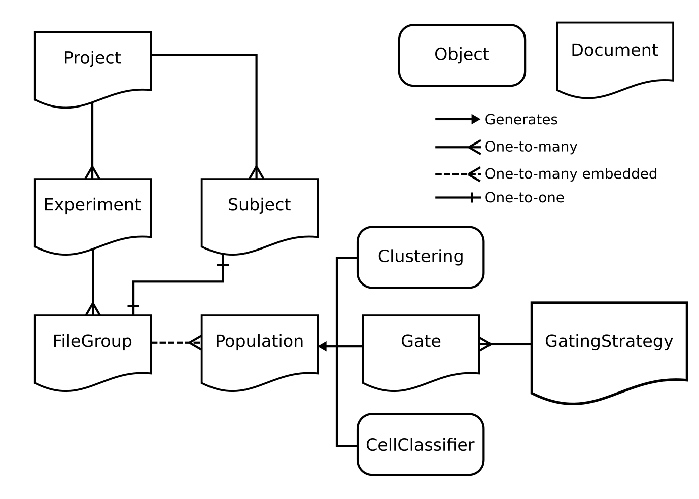
The CytoPy framework is built upon mongoengine an object-document mapper. Without going into too much detail, each of the documents in the figure above has it’s own class that we can interact with. For the most part, the user only needs to be concerned with the Project class as the user will use the methods of this class to access all other documents.
A brief summary of the documents and other objects from the figure above is given below:
Project: the central control of CytoPy’s database and the first thing a user will create when starting a new project. This document is used to create all other documents within the database and to access data as we go back and forth in our analysis.
Subject: for each biological entity in our study e.g a patient, cell line, mouse etc, we create a Subject to house any additional meta data. This document is completely dynamic and has no restriction as to how we store data within it.
Experiment: from our Project we create Experiment’s, one for each unique set of staining conditions we are investigating. The Experiment handles standardisation of cytometry data as it enters the database. We use an Experiment to create and add FileGroup’s.
FileGroup: a FileGroup stores the cytometry data associated to a single biological specimen. The FileGroup must contain one file that represents the primary staining of the biological specimen and can additionally store any number of files representing controls such as FMO’s or isotype controls.
Population: embedded within each FileGroup are Population’s. These documents define the index of events that pertain to a group of phenotypically similar events. Every FileGroup starts with one Population by default called ‘root’ that holds the index for every event in the primary staining. Population’s are generated by Gate, Clustering or CellClassifier.
Gate: the Gate document provides a persistent data structure that defines a manual or autonomous gate. Similar to traditional gating performed by software like FlowJo, the Gate document can generate a geometric object in one or two dimensions that encapsulates the members of a Population.
GatingStrategy: we never interact with Gate documents independently but instead construct them using the GatingStrategy. This defines a sequence of Gate documents and how they should be applied. The GatingStrategy can then be saved to the database and applied to data ad-hoc.
Clustering: another popular strategy for categorising cytometry events is to applying clustering algorithms in high-dimensional space; that is, apply these algorithms to all available events and parameters. The Clustering class is an algorithm-agnostic tool that enables you to apply any clustering algorithm to one or many FileGroup(s) and generate Population’s. This class also provides functionality for meta-clustering to match clusters between FileGroup’s.
CellClassifier: CytoPy offers another strategy for categorising cells and this is using supervised machine learning. A FileGroup with existing Population’s can be used as training data for any supervised classifier within the Scikit-Learn ecosystem, including XGBoost. Additionally, the Keras Sequential API can be used to define deep neural networks.
Note
Do Populations store control file indexes? No, instead CytoPy makes the assumption that primary staining and controls are collected under the same conditions. Therefore, the Population’s in the primary data serve as ideal training data to predict the Population’s of control samples. Therefore, when we request a Population of a control file in a FileGroup, CytoPy uses supervised classification to estimate this Population.
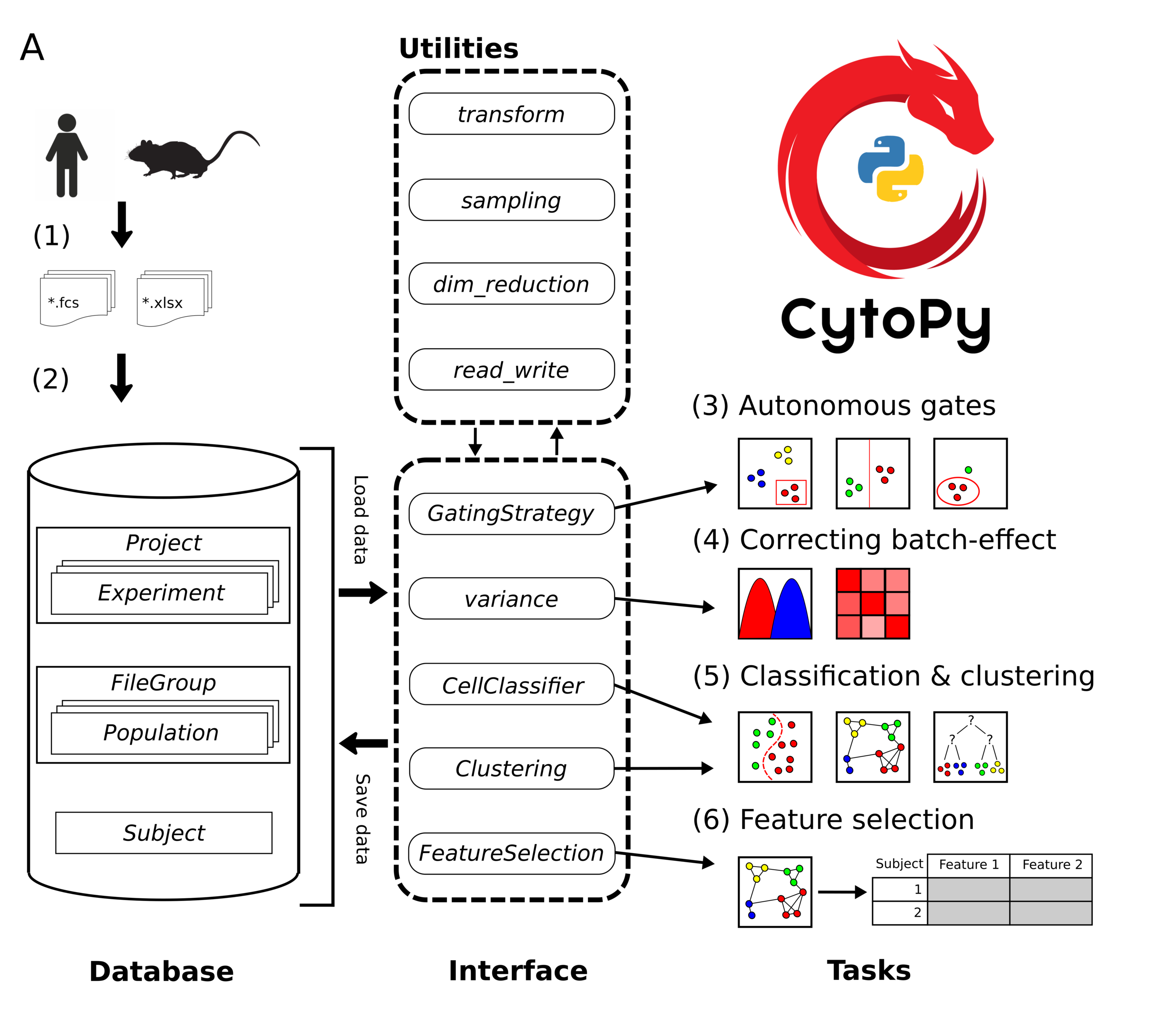
There are additional tools and utilities within the framework, notably the variance module for assessing and correcting batch effect, the plotting module for various plotting functions, the transform module for transforming and scaling data, and the feature_selection module for feature extraction, inference testing, and feature selection. A summary of the recommended pathway for analysis is given in the image below, however the individual modules of CytoPy can be used independently:
Connecting to the database
The first step in any analysis is to connect to a database. We don’t have to initialise a database or even create a schema. When we connect to a database for the first time, it is automatically generated if it does not exist.
We connect to a database using the global_init function from cytopy.data.setup. Connections are registered globally, so you only have to call global_init once per session. If working locally you just can name the database:
from cytopy.data.setup import global_init
global_init('MyDatabase')
Now the first time that we commit something, a new database will be created with the name “MyDatabase”. If the database is stored on some remote server we can pass additional arguments to global_init:
global_init('MyDatabase', host='192.168.1.35', port=12345)
# With authorisation
global_init('MyDatabase',
            host='mongodb://localhost/production',
            username='admin',
            password='12345')
Setting up a Project
Once we have a database connection, we can create a Project. We need to provide a name for the project and where we want to store the cytometry data. The cytometry data is stored as HDF5 files on your local drive and mapped to meta data in MongoDB:
# We store HDF5 files on our local drive and provide the path to 'data_directory'
from cytopy.data.project import Project
new_project = Project(project_id='TestProject',
                      data_directory='/home/user/CytoPyData')
new_project.save()
We now have a Project to work with and has been committed to the database by calling the save function. Since our Project is a mongoengine document we can retrieve it from the database using their query API:
new_project = Project.objects(project_id='TestProject').get()
We can use this API to list existing Project’s:
# Returns a list of Project documents
Project.objects()
If we need move the HDF5 data at a later point, this should be done with the update_data_directory function:
new_project.update_data_directory('/home/user/new/path')
Warning
The update_data_directory will move the existing directory by default, it is advised not to move this directory manually.
Adding Subjects and meta data
For each project we will have biological entities we are studying and collecting biological material from e.g. mice, humans, cell lines etc. To keep track of meta data about each subject in our study we add Subject documents. This document can also house data that is not sourced from cytometry e.g. plate based assays or mass spectrometry.
We create a Subject using the add_subject function of Project*:
# We don't have to call save as it is invoked automatically
new_project.add_subject(subject_id="Our first subject")
The only required field is the subject_id but we can pass any number of additional keyword arguments to create additional fields. They can be of any type and we can add embedded fields by passing nested dictionaries. Here is an example of a slightly more complex Subject:
new_project.add_subject(subject_id="Complex",
                        age=43,
                        gender="Male",
                        infection_data={"source": "Blood culture",
                                        "Isolates": [{"name": "E.coli",
                                                      "type": "bacteria"},
                                                     {"name": "Candida albicans",
                                                      "type": "Fungus"}]},
                        elisa_data={"TNFa": 25.3, "IFNg": 13, "IL6": 34.3})
This subject will contain the fields ‘age’, ‘gender’, ‘infection_data’ and ‘elisa_data’. Both ‘infection_data’ and ‘elisa_data’ are embedded fields that have additional fields within them as a nested tree.
We can edit and delete a Subject by retrieving the document from the Project and then acting on that Subject:
complex_ = new_project.get_subject(subject_id="Complex")
# Add a new field
complex_["diseased"] = True
# Edit a field
complex_["age"] = 41
# Always make sure to save our changes
complex_.save()
# We can delete the subject. It will automatically be removed from our project
complex_.delete()
Adding an Experiment
To add cytometry data we have to create Experiment’s, one for each unique set of staining conditions in our Project. An Experiment defines the markers and stains used and standardises cytometry data at the point of entry.
The problem with cytometry data collected over a long period of time is that you inevitably end up with inconsistencies between file meta data. This is most problematic for channel and marker names. An example is shown below with two files with the same staining but differing marker names for CD16 and live/dead stain:
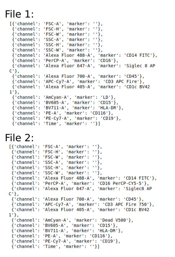
Note
We can inspect the channel/marker mappings of an FCS file using the cytopy.data.read_write.fcs_mappings function
To overcome these complications, all data is normalised upon entry into the database. An Excel template should be provided with two sheets:
mappings - expected channel/marker mappings with standardised names to be applied to all files under this staining panel
nomenclature - how to identify a channel/marker so that it can be standardised
There are examples provided in the Peritonitis analysis notebooks (https://github.com/burtonrj/CytoPy_Manuscript) and a template can be found in the CytoPy github repository.
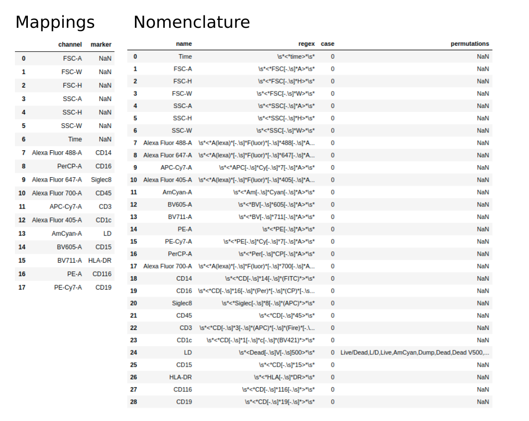
The mappings sheet contains two columns, channel and marker, with each row specifying a valid pairing. Where a channel does not have a corresponding marker (and will therefore be referred to using the channel name in analysis) the marker column should contain a null value.
The nomenclature sheet contains four columns. The first identifies each channel/marker. Channels and markers are identified and standardised using the regex column and/or the permutations column. The regex column contains a regular expression used to identify a pattern corresponding to the standardised channel/marker name.
For those unfamiliar with regular expressions, or for cases where the variability of a channel/marker naming can make regular expressions hard to manage, the permutations column can be used. Permutations of the standard channel/marker name can be provided as a comma separated string, where a channel/marker will be matched to the standardised name based on a like-for-like match to any of the substrings (separated by a comma).
The case column is simply a boolean value that, when true, makes the search case sensitive.
Below we see an example of these two sheets:
Once we have a template we’re happy with, we can create an Experiment like so:
new_experiment = new_project.add_experiment(experiment_id="First Experiment",
                                            panel_definition="/path/to/template.xlsx")
The Experiment is automatically created, associated to our Project and returned to us in the new_experiment variable. If we want to load the Experiment back into our environment we use the get_experiment function of Project:
new_experiment = new_project.get_experiment("First Experiment")
We use the delete_experiment function to remove an Experiment:
new_project.delete_experiment("First Experiment")
This automatically commits this change to the database and will also delete associated FileGroup’s.
Adding cytometry data
Now we have an Experiment we can start adding our cytometry data. Cytometry data can be added using Flow Cytometry Standard files (fcs) version 2.0, 3.0 or 3.1. Alternatively, cytometry data can be added using a Pandas DataFrame, allowing data to be imported into CytoPy using various other formats e.g from HDF5 or csv files.
Data is added to an Experiment using either the add_fcs_files or the add_dataframes method, depending on the input source.
Note
The data itself is stored in CytoPy as raw untransformed values. This is because transformations are applied during analysis rather than during data entry, to allow the user to experiment with different data transforms. Available transforms to apply during any analytical process (found in cytopy.flow.transforms) are:
Inverse hyperbolic sine transformation
The transform module also contains convenient methods for normalising and scaling data using the Scikit-Learn catalogue.
For convenience, we can use the get_fcs_file_paths to find the absolute paths for FCS files associated with a single biological specimen:
from cytopy.data.read_write import get_fcs_file_paths
fcs_paths =  get_fcs_file_paths("/path/to/specimen/directory",
                                 control_names=["control1", "control2"],
                                 ctrl_id="FMO",
                                 ignore_comp=True,
                                 exclude_dir="DUPLICATE")
In this function we provide the path to the folder containing the FCS files for a single biological specimen. We provide the name of control files and a ctrl_id which is a keyword used to identify files that are controls i.e. the file name must contain ‘FMO’ to be considered a control file. We’ve also said to ignore filenames containing the term “compensation” and will ignore subdirectories containing the term ‘DUPLICATE’.
The function expects a single primary staining file (identified by the absence of the control ID term) and will raise a warning otherwise.
This function returns a dictionary with the keys ‘primary’ and ‘controls’, with values corresponding to the absolute paths to the FCS files.
With the FCS files we can create a FileGroup to house them:
primary = fcs_paths.get("primary")[0]
controls = fcs_paths.get("controls")
controls = {x: v[0] for x, v in controls.items()}

new_experiment.add_fcs_files(sample_id="New File",
                             primary=primary,
                             controls=controls,
                             subject_id="Subject 1",
                             compensate=True,
                             verbose=True)
This method takes the following arguments:
sample_id: Unique sample identifier (unique to this Experiment)
primary: File path for primary staining single cell cytometry data
controls: dictionary of filepaths/FCSFiles for single cell cytometry data for control staining e.g. FMOs or isotype controls
compensate: If True, the fcs file will be searched for spillover matrix to apply to compensate data. If a spillover matrix has not been linked to the file, the filepath to a csv file containing the spillover matrix should be provided to ‘comp_matrix’
comp_matrix (optional): Path to csv file containing spill over matrix for compensation
subject_id (optional): If a string value is provided, newly generated sample will be associated to this subject
verbose (default=True): If True, progress printed to stdout
processing_datetime (optional): Optional processing datetime string
collection_datetime (optional): Optional collection datetime string
missing_error (default=”raise”): How to handle missing channels (channels present in the experiment staining panel but absent from mappings). Should either be “raise” (raises an error) or “warn”.
Accessing data
We access our data using the Experiment as a portal to our FileGroup’s. For the most part we can use the various tools in CytoPy and we don’t have to touch FileGroup’s directly, but we can if we want direct access to our data.
To access a FileGroup we go via our Project and Experiment:
new_project = Project.objects(project_id="TestProject").get()
new_experiment = new_project.get_experiment("First Experiment")
file_data = new_experiment.get_sample("New File")
To access the complete data as a Pandas DataFrame we use the data method:
# Primary staining
data = file_data.data(source="primary")
# Primary staining down sampled
data = file_data.data(source="primary", sample_size=5000)
data = file_data.data(source="primary", sample_size=0.5)
# Control data
data = file_data.data(source="control1")
To get the data of a particular population we use the load_population_df. The ‘root’ population is generated by default whenever a FileGroup is created and indexes all the events in the primary staining:
root_data = file_data.load_population_df(population="root", transform="logicle")
This grants us access to the population data of primary staining but to access controls we use the load_ctrl_population_df. This estimates the control population using the primary staining as training data:
ctrl_data = file_data.load_ctrl_population_df(ctrl="control1",
                                              population="pop1",
                                              classifier="XGBClassifier")
Deleting data
Deleting data is simple, we can use the delete method for most documents and this echos to associated documents automatically.
When we want to delete populations we can either use the delete_populations method of the FileGroup containing the populations.
Examples
We provide examples of setting up experiments with the Jupyter Notebooks that accompany our manuscript:
Setting up FlowCAP
Setting up the Peritonitis project
The original Peritonitis dataset can be obtained from this link: https://drive.google.com/file/d/1y6qL_7l2unDoUkNqlr9Xqubq5_sP1E14/view?usp=sharing